We use cookies to help us provide you with a more enhanced and personalized experience adapted to your interests. By using our site you agree to our Terms of Use and Privacy Policy, including our use of cookies.
To read the audio transcript for The Last 100 Meters of Fiber to and Into the Home click here.
AN OFS WHITE PAPER: NEW TECHNOLOGIES ENABLE FASTER, EASIER FIBER INSTALLATION INTO HOMES AND MDUs
For immediate access to our exclusive FTTH whitepaper, click here.
EZ-Bend Cabling and InvisiLight Solutions enable fast, easy and accepted fiber deployments to and into MDUs, homes and offices.
Executive Summary
Driven by unprecedented demand for Gigabit and fast emerging 10 Gigabit Broadband, Fiber to the Home (FTTH) deployment is expected to reach record numbers in the coming years. According to iDate, FTTH connections will more than double in Europe over the next six years, while RVA forecasts that FTTH investment in North America will double in the next five years compared to the previous five. In addition to homes, service providers are bringing fiber to the living unit in multiple dwelling units (MDUs) and into commercial and institutional buildings. In all these scenarios, a cost-effective and compact optical network terminal (ONT) is typically placed inside each living unit or office to enable Gigabit or even 10 Gigabit connectivity. However, there are aesthetic and cost challenges to placing fiber inside residences or buildings. While service providers typically prefer to deploy ONTs deep within subscribers’ units with co-located Wi-Fi:
there may be no existing fiber ducts or pathways to the ONT location.
installing new ducts or cutting and patching walls can be very expensive and disruptive.
surface mounting conventional fiber cables can be unsightly and result in optical signal loss when the cables are bent around the many sharp corners on the pathway to the ONT.
wire molding or tape systems to house fiber are typically cost prohibitive, visible. and very slow to install.
Transcript:
Good day, my name is John George. I’m Senior Director of Solutions and Professional Services with OFS. Today I want to share what’s new in my world that could help you build better fiber to the home (FTTH).
Originally, FTTH deployments were fiber to outdoor ONTs on the side of a house. From there, copper typically was used to reach an indoor residential gateway inside the home. Over time we discovered indoor ONTs are smaller, and less expensive. They could be deployed inside the home, co-located with the wi-fi in the center of the building and achieve much better wi-fi coverage. This would reduce the cost, but there had to be a way to get the fiber into the home to that indoor ONT.
For MDU’s and apartment buildings, it evolved from fiber to the building, and trying to use the existing in-building copper to bring the internet service to each living unit. That proved to be insufficient from a bandwidth perspective for MDUs. To support 10 gigabit data rates that are being deployed now, it’s desired by service providers to get fiber into each living unit of an apartment building.
I’ll walk you through some innovative technologies we offer, that help solve those significant problems. The first one is EZ-Bend Cabling Solution. This is a three-millimeter diameter cable. It can have connectors on both ends. It can simply be stapled around any corner, and bends sharply in half with no concern about loss whatsoever. It has a 2.5 millimeter minimum bend radius – that’s twice as tight as anything else you can get on the market. The best from others is only five millimeters.
The EZ-Bend 2.5 millimeter bend radius technology is even more necessary as we move to from gigabit, to 10 gigabit. 10 gigabit use longer wavelengths in the transmission system. Longer wavelengths have much higher bend loss than what’s used for the gigabit. So, cable bends in a 10 gigabit transmission is a bigger challenge, but we solve it with the EZ-Bend. You can literally bend it any way without concern for signal loss.
The next technology we offer is the OFS InvisiLight Solution. It‘s used to solve issues inside the home or apartment. Originally, stapling cables inside the home was acceptable. Now, many customers don’t want to see the fiber at all inside the living unit. The OFS InvisiLight Solution is fiber installed inside an apartment, or home that blends into its environment; nearly invisible to anyone looking directly at it. The OFS InvisiLight Solution gets the fiber deep inside to the ONT. We have connectors on both ends of the InvisiLight spool making it easier to deploy a single part number, that can cover up to 132 feet, getting fiber into a home or an MDU living unit.
We also have a 12 fiber version, and a 16 fiber version for MDU hallways. These editions to go down the hallway and drop off the single fiber InvisiLight into the living unit.
Finally, we have the EZ-Bend Single Family Drop Solution that includes drop cabling, from the pole or pedestal to the home, and into the home. This is a double end connectorized assembly that’s toneable orange and can be laid out as a temporary drop, then buried later. What’s beautiful about this is it has the InvisiLight fiber inside the cable, so you can run this to the house below grade, direct buried, or induct, then wrap the house with it, and then to extend into the home to reach the ONT. All that is needed is to strip the jacketing off and then what you have is the fiber outside going through the wall to the inside where we’ve got the InvisiLight deployed to the ONT. Essentially this is a single piece of glass all the way from the curb, into the home, and into connecting the ONT. Quite simple, one part number, you don’t need a Network Interface Device (NID). You don’t need the time to install the NID. You save dollars if you avoid conduit and the NID by going with the EZ-Bend Single Family Drop Solution to the home into the home straight to the ONT.
That’s what’s new in my world. Thank you for listening.
We invite you on a tour of our fiber optic cable manufacturing facilities in Carrollton, Georgia, USA. View the highly automated OFS manufacturing process that produces a wide variety of fiber optic cables and products for telecommunications applications. Loose tube, microcables, flat ribbon, ADSS, ultra high density rollable ribbon cables and premise cables are all made here.
What is Fiber Optic Cable Made up of?
Fiber optic cables are made up of several components: a core, cladding, jacket, and strength members.
The core is the optical fiber itself which is a continuous strand of ultra-thin glass.
Within the core, there are two highly specialized glass coatings called cladding and jacketing.
The cladding helps bounce back imperceptible light signals as they travel along the cable by reflecting off of its walls.
The jacketing protects the delicate optical fibers from mechanical damage and environmental effects.
Lastly, strength members such as aramid yarns or steel wires are used to reinforce and protect the cable further against bending or stretching forces. Together these components form a fiber optic cable that carries light signals over long distances without signal loss or interference.
The manufacturing facility is registered in compliance with the ISO 9001, ISO 14000, and TL 9000 standards. Traceability is maintained through every step of the process and ultimately back to the incoming fiber. The facility also has a fully functional product qualification lab and cable installation test track.
OFS Uses Both 200 and 250 Micron Fibers
OFS makes several different fiber structures in the Carrollton facility, including loose tube, flat ribbon and rollable ribbon structures. These structures are used in different cable types and applications.
Statistical Process Control Techniques
Each stage in the manufacturing process is highly controlled with appropriate dimensional targets and tolerances.
Colored ink is applied to the Fiber
The industry standard color code is used to provide clear identification of the fibers over their lifetimes. Colored ink is applied to specified thicknesses, cured, and respooled for the next step in the process.
Buffer Tube Manufacturing Process
To make loose tubes, fibers or ribbons are paid off of their spools and a buffer tube is extruded around them. The Carrollton plant makes gel-free and gel-filled buffer tubes of different materials, including polypropylene and PBT. Different sized buffer tubes are used for different product types. Buffer tubes used in outside plant applications include either water blocking materials impregnated with super absorbent polymer or gel.
Ribbon Manufacturing Process
A matrix material is applied to the fibers to bind them together so they can be spliced as a group. 12 and 24 fiber flat ribbons are most common. Fiber color code alignment and geometric specifications are very important so ribbons can be spliced and connected in the field.
Rollable ribbons are only partially bonded together, enabling them to be rolled into a cylindrical package. Rollable ribbons are only partially bonded together, enabling them to be rolled into a cylindrical package. Since circles are more space efficient than rectangles, rollable ribbons cables can hold twice the fibers as comparable sized flat ribbon cables. Since these fibers are partially bonded, they can be easily spliced either as single fibers or as a ribbon, giving more deployment flexibility to the network operator.
Cabling
OFS makes two main types of cables – stranded cables and central tube cables.
Stranded cables are made by stranding tubes of fibers, flat ribbons, or rollable ribbons around a central member. Stranded cables are often used in applications requiring frequent access to fibers.
For direct-buried cables, one or more steel armor layers may be added to provide rodent resistance and toning capability.
Outer Jacket
Different versions of polyethylene are used for the majority of outside plant cables. For inside plant or indoor/outdoor cables, materials are chosen to include appropriate flame and smoke resistance.
Information Printing
Type of cable, date of manufacture, length and a unique serial number that can enable traceability through the manufacturing process is printed.
Final Testing
Once manufacturing is complete, the finished cable undergoes final testing for length and optical properties.
Shipping
Cables are then packaged for shipment and loaded on trucks to their final destination.
The first Article in this series focused on growth in bandwidth demand and attenuation in optical fibers. Article 2 concentrated on the several types of dispersion that exist in fiber today, closely followed by Article 3 – Fiber strength and reliability. Article 4 featured single-mode fiber geometries and now the latest release from OFS – Article 5, deals with “Cut-off Wavelength” (COW). This latest article will help the user to understand what “cut-off wavelength” is, why does it matter and how is it measured.
CUT-OFF WAVELENGTH MAKES A COMEBACK IN IMPORTANCE
Take an intro to fiber course, and you’ll learn about attenuation, dispersion, fiber geometry, maybe fiber strength. However, buried in the fine print of fiber specs is a parameter called cutoff wavelength. Although fiber manufacturers and some fiber users are aware of cutoff wavelength, it’s not as famous a parameter. Users still focus primarily on attenuation, maybe dispersion, as critical propagation properties.
Due to relatively new operating wavelength requirements below 1310 nm, some astute end users are taking a renewed look at cutoff wavelength specifications. Relatively new Passive Optical Network (PON) protocols are looking at wavelengths as low as 1270 nm, which, optical spectrum-speaking, is a hop and a jump away from the historical cable cutoff wavelength specification λcc, 1260 nm.
Different fibers do different jobs in today’s networks. Some fibers are bend insensitive. Some fibers enable more power to increase signal-to-noise ratios at ultra-high speeds. Cutoff wavelength is important for the performance of these fibers, but these fibers may require differences in measurement methods versus “standard” G.652-type fibers. We’ll talk about measurement methods later in this paper.
WHAT IS CUT-OFF WAVELENGTH?
In an optical fiber a number of different light-“modes” may exist. Modes are different types of light waves which may each carry different portions of light from the input to the output of the fiber.
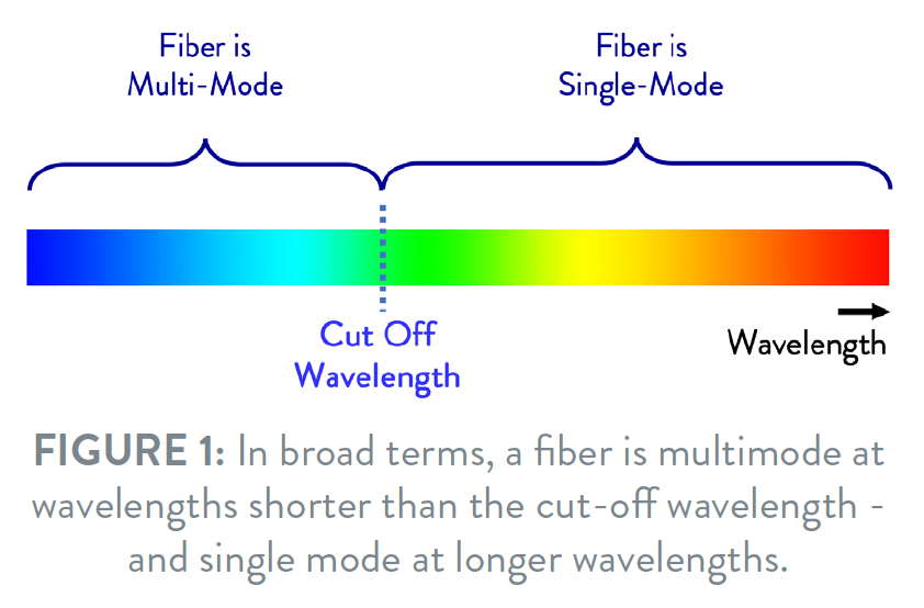
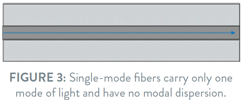
A multimode fiber, by definition, may carry several modes of light (several hundred), but in a single-mode fiber, only one mode is carried.
The wavelength at which the fiber is at the cusp of changing from single-mode to multi-mode is called the Cut-off Wavelength. Typically, a fiber is considered to be single mode for wavelengths longer than the Cut-off Wavelength (COW) – and multimode at shorter wavelengths. In real life, the transition from single mode to multi-mode transmission does not occur abruptly at an isolated wavelength – but rather relatively smoothly over a range of wavelengths. The single-wavelength number on a specification is a simplification.
The most common way to make a fiber single-mode is to reduce its core-size (diameter), but the contrast between the refractive index of the fiber core and the fiber cladding is also important. These two properties determine the “effective core size” which determines if the fiber is single mode or not at a given wavelength.
WHY IS IT IMPORTANT?
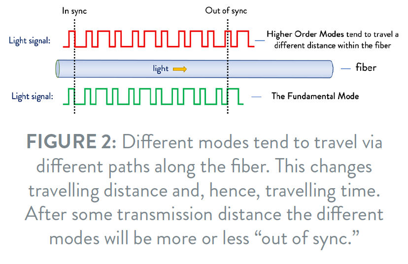
The whole idea of a single-mode fiber is to keep the other modes out of the optical transmission. The reason is why Multi-Mode fibers are used for short distance transmission only: different modes traveling through a fiber take different paths.
An optical pulse injected into a multi-mode fiber will be transmitted via different modes reaching the end of the fiber after slightly different travel times. Once the modes are recombined at the output of the fiber, the shape of the input pulse will have been distorted (blurred). This distorting effect on the pulse is known as modal dispersion and affects the bandwidth (MHz-km) of a multimode fiber. Single-mode fiber does not have modal dispersion, and consequently has much higher bandwidth over dramatically longer distances.
The concept of cutoff wavelength is receiving renewed attention as next generation PON systems begin operating at wavelengths shorter than 1310 nm. This will be discussed in more depth later in the paper.
“ONLY ONE LIGHT MODE IN MY SINGLE MODE FIBER, PLEASE!”
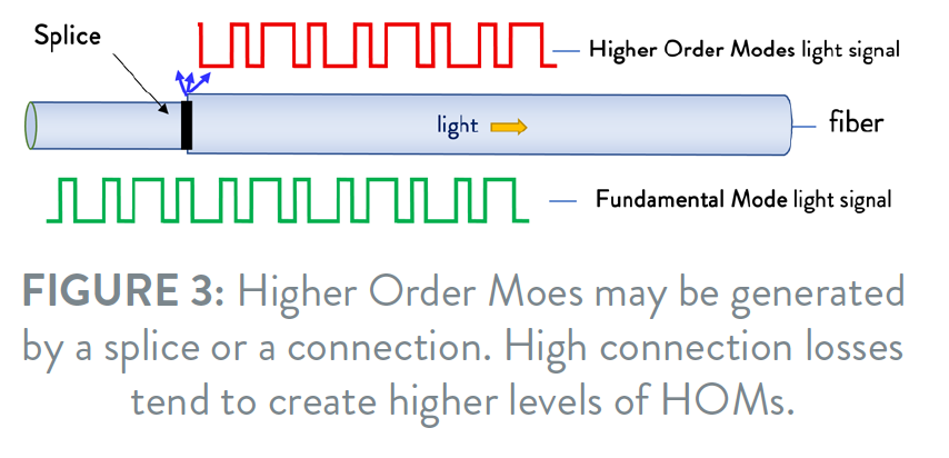
The light mode intended for transmission in a single mode fiber is called the Fundamental Mode (also called LP01). All other modes are called Higher Order Modes, the most important of those is the Secondary Mode (LP11).
And one might ask: “Where do those higher order modes come from?”
These modes may be generated at splices and connections between fibers. The higher the splice/connection loss, the more powerful the Higher Order Modes (HOM) tend to be generated.
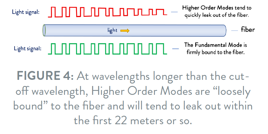
HOMs are also called “leaky modes” because they are bound only loosely to the fiber core and tend to leak out of the fiber after traveling a relatively short distance – for wavelengths longer than the Cut-off Wavelength. The longer the distance, the more of those modes will have leaked out.
The Cut-off Wavelength is defined as the wavelength at which the power level of the Higher Order Modes has been reduced by 19.3 dB relative to the level of the Fundamental Mode (strictly speaking this is true only for the Second Order Mode).
MODAL NOISE PROBLEMS
Do we need to worry about modal noise in today’s systems? Without wanting to raise unwarranted concerns, we want to highlight possible situations where modal noise may arise and be problematic.
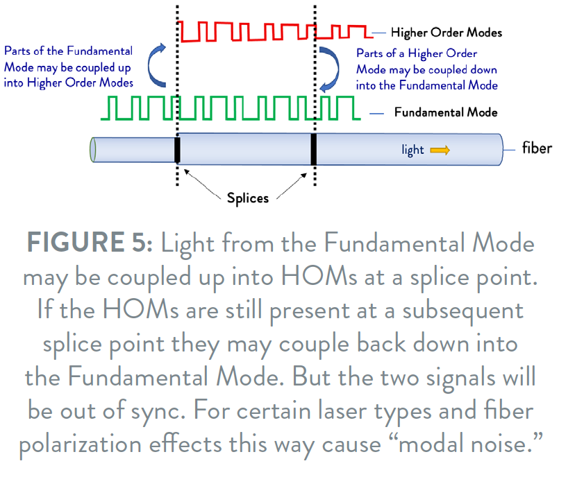
As briefly mentioned, splices or connectors will cause some of the light in the Fundamental Mode to be coupled into higher order modes. And likewise, light from Higher Order light modes may be coupled down into the fundamental mode by similar splices or connectors.
Situations may arise where two splices or connectors are situated closely to each other. If they are too close, or if the Cut-off Wavelength is too high, parts of the HOMs generated at the first splice/connector may be coupled back down into the Fundamental Mode at the second splice/connector and mixed with light from the initial Fundamental Mode.
This may cause a problem because the travelling time for the light signal may typically be different in the Higher Order Modes than in the Fundamental Mode – and so the two signals may be somewhat out of phase when mixed together. Because of polarization and other effects, such phase difference may change as a result of temperature variation and stress, and this can result in a type of noise called Modal Noise.
To create significant levels of modal noise two joints with large connection losses must exist (one is not enough). Furthermore, the two joints must be so closely spaced that Higher Order Modes have not leaked out of the fiber before reaching the second joint. And finally, the laser used must exhibit some level of mode partitioning.
WHY ARE THERE DIFFERENT TYPES OF CUT-OFF WAVELENGTH?
The Cut-off Wavelength of a fiber depends on the length of the fiber, the longer the fiber the lower the Cut-off Wavelength tends to be. For that reason, there are 3 types of Cut-off Wavelengths defined to match different applications:
CABLE CUT-OFF WAVELENGTH (λcc): It is very easy to mistake this term for “Cabled COW” – but in principle it does not really matter whether the fiber is cabled or not. The initial intention with this parameter was to simulate a situation with two closely spaced cable splices, for example in a repair situation. 20 meters splicing distance was considered a relevant minimum – and to simulate fiber being deployed in splice cassettes, a 1-meter fiber length including one 80 mm loop was added in each end for the measurement set up. Effectively the full length of the fiber measured is 22 meters.
JUMPER CUT-OFF WAVELENGTH (λcj): As the name suggests it simulates a jumper cable. It is measured on a 2-meter length of fiber with one winding which diameter may be freely defined – which in the US is typically 152 mm.
FIBER CUT-OFF WAVELENGTH (λcf): As the name suggests it simulates a fiber being bent in only large diameters. In principle it is measured on a 2-meter length of fiber with one 280 mm diameter, but as explained later special care must be taken during measuring – especially for bend-insensitive fibers.
Because Cable COW is measured on a 22 m fiber sample whereas Fiber COW is measured on 2 m fiber, Fiber COW is typically higher than Cable COW.
Normally it is possible to find a good statistical correlation between the Cable COW and the Fiber COW. Since only 2-meter fiber is needed when measuring Fiber COW, it is easier to measure Fiber COW than Cable COW where 22 meters are needed. And because of the correlation Fiber COW measurements are often sufficient to ensure that the Cable COW is within limits.
Also, cabling fibers often has an effect of stripping out higher order modes, due to either macro or micro-bending of the fibers inside the cable sheath. In situations where this effect is significant, Cable COW measured on a cabled fiber may be lower than Cable COW measured on a non-cabled fiber (and of course lower than Fiber COW).
It depends on the fiber type and design, but a realistic example for a step-index fiber is a fiber cutoff of 1350 nm could have a corresponding cable COW of 1260 nm.
WHY IS CABLE CUT-OFF WAVELENGTH SPECIFIED AS 1260 nm IN IEC AND ITU-T RECOMMENDATIONS?
Initially Single Mode fibers were intended for 1310 nm operation, and manufacturing variability of lasers were rather large, so lasers sold as “1310 nm lasers” could in fact emit light at rather different wavelengths than 1310 nm. So, to create a certain “guard band”, the maximum Cable COW was defined to be 1260 nm.
Today, laser wavelengths may be more tightly controlled and extremely accurate, but those lasers may also be more costly than less accurate lasers. Furthermore, some FTTH/PON transmission formats (especially newer ones such as XGS-PON) use wavelengths close to 1260 nm. So, the 1260 nm COW today has renewed relevance.
BEND-INSENSITIVE FIBERS – AND PROBLEMS MEASURING THEIR ATTENUATION
This may seem like a subject entirely different from Cut-off Wavelength – but measurement problems are quite similar and may not be obvious at all.
To determine the Cut-off Wavelength, two measurements of the power on the output of the fiber are compared:
A. Power in the Fundamental Mode (LP01) only
B. Power in the Fundamental Mode (LP01) and the Higher Order Modes (which in practical terms means the Second Order Mode: LP11)
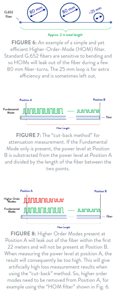
“B” is just a simple measurement of output of the fiber – including all modes. But in order to measure “A” we need a filter to get rid of the Higher Order Modes. They are loosely bound modes, and in a standard G.652 fiber they will tend to leak out of the fiber relatively quickly – especially when the fiber is bent in small diameter loops. Two 80 mm loops – perhaps with an added 25 mm loop – in a 2-meter G.652 fiber will do the trick, so this is often used as a HOM filter.
MEASURING ATTENUATION USING THE CUT-BACK METHOD
When measuring the attenuation of a Bend Insensitive fiber – including some advanced Large Area G.654 fibers – different methods may be used. The Cut Back measurement method is often considered the reference method. Light is injected into the Fiber Under Test (FUT) and the aim is to measure the power injected into the fiber (at the beginning of the fiber) and compare that to the measured power at the end of the fiber. Subtract the two and the fiber attenuation is found – divide this by the fiber length, and the attenuation in dB/km is found.
To determine the exact input power level, the fiber is often cut a short distance from the actual input end of the FUT, and the input power level is measured.
It is always important to avoid Higher Order Modes at the input of the measured fiber, since they will leak out of the FUT over a relatively short distance and be missing at the output of the FUT. HOMs are like ghosts – appearing at the input of the FUT and then disappearing along the fiber length. With these around, one would tend to measure a “too high” power level at the input of the fiber – and the resulting calculated fiber attenuation will then be too high. Such increased attenuation will tend to be more pronounced at shorter wavelengths.
Previously, such attenuation measurements were predominantly made on standard G.652 fiber and that was easy. You could grab the first 2 meters of the G.652 FUT, make the desired 2 or 3 loops directly on the fiber itself within those first 2 meters of fiber and that would give you your HOM filter and get rid of the Higher Order Modes. Your cut-back point for attenuation measurement could then be situated right after the first 2 meters of the FUT – so you would only waste 2 – 3 meters of fiber for each measurement.
But on bend insensitive fibers it is not quite as easy to get rid of the higher order modes. These fibers tend to better restrict the light from leaking out during fiber bends. Unfortunately, that is true for the higher order light modes as well – those modes which we would want to get rid of when measuring the fiber.
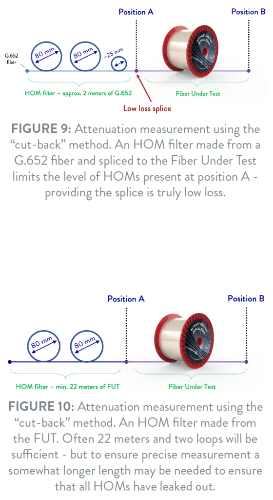
However, the 2-meter G.652 standard fiber with two 80 mm and one 25 mm loop may still be used. It may be spliced to the Fiber Under Test and if a good splice is obtained only an insignificant level of Higher Order Modes may be generated at that splice point – ensuring a good measurement if the splice point is also used as the Cut Back Point.
Another possibility is to use the first 22 meters of the FUT including the two loops of 80 mm recommended for measuring Cut-off Wavelength. Since that is the recommended test set up for COW measurement, you know that after 22 meters the HOM level is very low at the FUT’s COW or longer wavelengths. The Cut Back Point may be chosen to be just after the first 22 meters of the FUT but if very high precision measurement is required, or if FUT is relatively short, more than 22 meters may be needed.
On OTDR measurements problems caused by HOMs are often hidden. The reason for this is that an OTDR will typically have a “Dead-Zone” during which the light detector of the OTDR is recovering and as such unable to detect the incoming light signal. This may cover some 500 meters during which length the HOMs have since long leaked out of the fiber.
Hi, I’m Mark Boxer Technical Manager for Solutions and Applications Engineering for OFS and this is what’s new in my world.
We are seeing a tremendous amount of recognition around the country that fiber is the answer for connectivity now and into the future. We’ve seen just unprecedented interest in fiber networks around the country and the benefits that bandwidth brings to an area and specifically with a focus in rural areas. I live in a rural area this is an old, restored farmhouse and we are seeing a lot of interest in broadband even in very remote and rural areas. The Fiber Broadband Association is in the process of publishing some projections showing that demand for a household will exceed a gigabit per second.
This demand is coming from a lot of different places. It’s coming from the use of high-resolution video, all of the different applications that we’re running, as well as augmented reality and virtual reality. We’re starting to see a lot of these trickle into daily life today. We expect that these types of technologies will continue to get more accepted over the decade leading to a lot of increase in demand for bandwidth. Fiber is really the only way to build a future proof network. We are also seeing a high level of interest in next generation PON platforms including XGS-PON, NG-PON2. These are platforms that use different wavelengths than the networks that we’ve been deploying primarily for the last 15 to 20 years. These wavelengths are a little bit different because they are a little bit longer and they’re also a little bit more bend sensitive. Which means that we’re also a little bit more focused on bend sensitivity and making sure that these networks are viable for decades to come as more of these applications and more of these protocols come online and onto the networks.
If you’ve been using OFS fiber for years you know this is something you’ve probably heard about for a long period of time. It’s something your network is well prepared for. There has been lots of innovation especially over the last few years with fiber. There have been some groundbreaking technologies introduced and one of those is the concept of rollable ribbon. We see rollable ribbon making its way really into all parts of the network and we think that’s going to bring a tremendous amount of benefits to network operators including higher density. Once you have higher fiber density you can put more fibers into a smaller space. That frees up a lot of benefits with underground networks because you can pack more fibers into a smaller duct. For aerial networks now you can go longer distances with less sag or less weight on your poles so a lot of different benefits there. Also, since it’s a ribbon then you get the benefit of ribbon splicing.
We’re seeing a lot of interest in rollable ribbon being applied throughout the network and on top of that we’re seeing a lot of interest in builds to the home, builds to the MDU. These networks have a lot of bends and so they require that their fibers have a lot of bend insensitivity and so we’ve seen a lot of builds of those kinds over the last six months to year.
At OFS we bring a lot of different solutions. If you’re a network operator don’t get overwhelmed that you have to use this technology or that technology. A lot of these are just different tools in the toolbox and you can mix and match to make your network the most sustainable and viable for the for the future and OFS can really help with that.
So, one of the things that we are happy to do is spend some time with you looking at the choices that go into the network. So if you’re interested in learning more about some of the choices and the trade-offs in their network and how we could potentially help with that please feel free to contact me or your OFS representative and we’d be happy to help.
The first Article in this series focused on growth in bandwidth demand and attenuation in optical fibers. Article 2 focused on several types of dispersion that exist in fiber, followed by Article 3 – Fiber strength and reliability.
This article, the fourth in the series, will focus on single-mode fiber geometries.
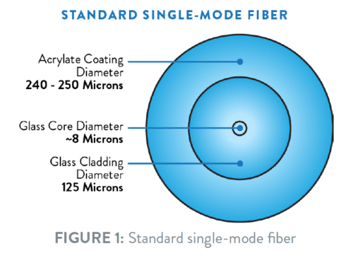
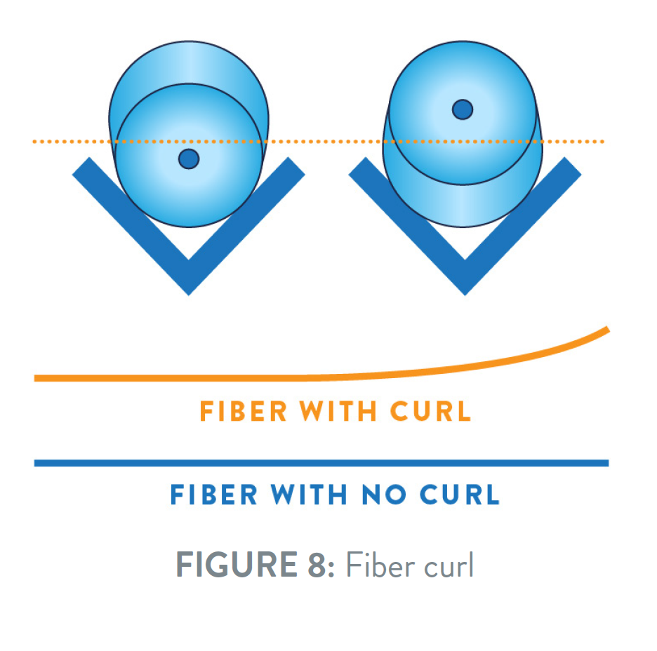
When speaking about fiber geometries, we typically consider diameters of core, MFD (Mode Field Diameter), cladding and coating. Also, the concentricities of those and the ovalities – and then the actual curl of the fiber. More on that later however.
The primary impact of fiber geometry occurs in the splicing and connectorization processes. Fibers with good and consistent geometry tend to splice and connect better with lower connectorization losses than do others. However, as highlighted previously in Article 2, fiber concentricity could also play an important role for polarization mode dispersion (PMD) performance and is an important parameter. For high quality fibers geometry has been good for a long time, and we may have been so accustomed to it that we sometimes take it for granted. However, this may not always be the case.
We’ll work our way through a typical fiber specification, highlighting the importance of various single-mode fiber geometry specifications. In the first figure we present the basic properties of the geometry of a fiber.
CLADDING DIAMETER (OUTER GLASS DIAMETER)
Cladding diameter is the outer diameter of the glass portion of the fiber. For telecommunications fibers, this diameter has been 125 microns (μm) for a very long time. On the other hand, the diameter tolerance has not always been 0.7 μm.
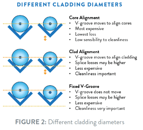
During the 1980s, optical fibers had outer diameter tolerances as high as +/- 3.0 μm. As illustrated in Figure 2, trying to match up 8 micron fiber cores when cladding diameters varied between 122 and 128 μm in diameter could result in very high losses, since the two cores may be significantly misaligned even though the claddings of the two fibers are perfectly aligned. This situation is why fusion splicing machines required additional technology to help align the actual fiber cores. This extra technology, however, increased the price of the splicing units.
As the industry matured, single-mode fiber diameters remained the same at 125 μm. However, over the same time period, the specification tolerance declined to 0.7 μm with typical variation along the length of the fiber becoming even tighter.
From a manufacturing perspective, such tolerances were not easy to achieve. When fiber was first invented, the developers had to create manufacturing methods along with ways to measure fiber diameter. When manufacturing to tolerances of tenths of a micron, inputs such as stray air currents, vibrations or particulate in the glass can cause significant diameter variability. These factors require top- tier fiber manufacturers to have very tight control over their processes and procedures.
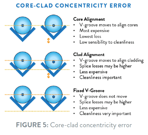
As diameter variability has decreased, splicing machines have reduced the alignment technologies needed. While there has been a significant decrease in the price of these machines, there has been no corresponding substantial increase in splice loss. Core alignment splicing machines still provide the best performance, however smaller “fixed V-groove” machines with lower prices and limited alignment capability have significantly reduced the performance gap. The typical splice loss for OFS AllWave®+ Zero Water Peak (ZWP) Optical Fiber, spliced using a core alignment splicing machine, is roughly 0.03 dB, whereas the same fibers spliced with a fixed V-groove machine have an average loss of approximately 0.05 dB. In a comparison of the absolute values, that is a significant difference. However, in the context of use in most fiber optic network applications, the difference is actually rather insignificant.
Enabled by tighter fiber geometry, the reduced cost of splicing machines is one of the factors that have contributed to the overall decrease in the cost of building fiber networks. In fact, this change has ultimately enabled fiber to the home to become a reality.
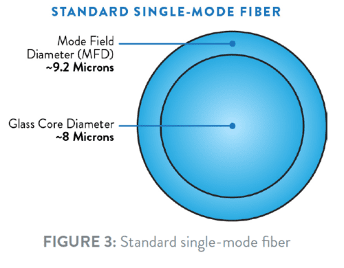
MODE FIELD DIAMETER (MFD)
Mode field diameter (MFD) is another specification related to fiber geometry. In a typical G.652.D- compliant single-mode fiber, not all of the light travels in the core; in fact, a small amount of light travels in the fiber cladding. The term MFD is a measure of the diameter of the optical power density distribution, which is the diameter in which 95% of the power resides.
MFD is important for two main reasons.
The first reason is that fiber bending loss is typically correlated with MFD. Unless special fiber designs are used, as the MFD increases, bend loss also increases, and vice versa. Historically, fibers with smaller mode field diameters are less bend sensitive. That being said, modern fiber designs has enabled fiber manufacturers to make bend insensitive, single-mode fibers with a nominal mode field diameter of 9.2 μm – which is the same as the vast majority of classical standard G.652.D fibers. However, there are also fibers with MFD as high as 8.6 micron offering superior bending performance, with very low bending losses even for bending diameters as low as 5 mm – which is half of the smallest bending diameter specified by ITU-T for G.657.B3 fibers.
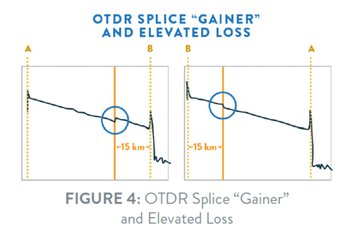
Second, because of the ease of use, OTDR measuring instruments are often used to measure attenuation. However, OTDRs only give correct results if the measurement conditions are perfect. A sudden jump in MFD is definitely not a perfect measurement condition. So in the case where two fibers of different mode field diameters are spliced together, the OTDR will errantly show either a power gain, known as a “gainer”, or elevated loss, depending on in which direction the measurement is taken. When measured from the larger MFD into the smaller, a gainer is produced. When measured from the smaller MFD into the larger, an elevated loss is seen, as shown below. This is an artifact of the OTDR measurement method and does not affect transmission properties. Breaking and re-splicing the fibers will typically not change the result, unless there’s a bad cleave or some other anomaly at the splice interface. The correct way to measure splices overall is bi-directional OTDR, which is even more important for fibers with MFD mismatches.
This fact shows why it may be advantageous to use bend-insensitive fiber with MFDs of 9.2 micron. Since experience with installation and measurements of fibers is almost always gained working with standard G.652.D fibers with MFDs of 9.2 micron, such bend insensitive G.657 fibers will behave in a very familiar way in terms of splicing and control measurements. Especially when splicing to the installed base of 9.2 μm MFD single-mode fiber.
CORE-CLAD CONCENTRICITY ERROR
Core/clad concentricity error (CCCE or CCE) is also called Core-Clad Eccentricity and measures how well the core is centered in the fiber. CCCE is measured in microns and, of course, the closer the core is placed to perfect center, the lower the CCCE value and the better it is. Again, core aligning splicers tend to give the lowest splice losses.
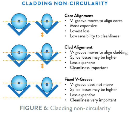
CLADDING NON-CIRCULARITY
Clad non-circularity is also called Cladding Ovality and measures a fiber’s deviation from being perfectly circular – becoming an oval rather than a circle. It is measured as a percentage difference between the “long” and the “short” diameter of an oval. If the Cladding Non-Circularity is zero the cladding forms a perfectly round circle. Similar to other fiber properties, better cladding non-circularity can result in improved splicing and connectorization performance.
FIBER COATING
While coating specifications are not as stringent as glass specifications, they are also important – especially when fibers are used in ribbons. The two main parameters are Coating Diameter (Uncolored) 237 – 247 μm and Coating-Clad Concentricity Error of max. 0.5 micron.
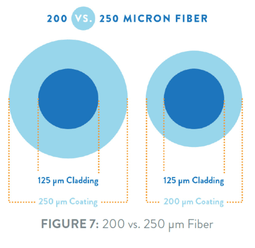
For roughly the first 30 years of single-mode fiber manufacturing, a coating nominal diameter of approximately 245-250 μm was standard in the industry. However, in 2014, OFS launched a 200 μm fiber in response to the need for higher fiber density in fiber optic cable designs.
Although the difference between 200 and 250 μm is not tremendously large, smaller diameter fibers can enable twice the fiber count in the same size buffer tube in a cable, while also still preserving long-term reliability. This fact has led to many new compact cable designs, including extremely small micro-cables, loose tube duct cables and all-dielectric, self-supporting (ADSS) aerial cables. As the demand for higher fiber density continues to increase, we can expect to see even more cable designs taking advantage of smaller diameter coatings. Important though, is that the coating will still be able to sufficiently shield the fibers from micro-bending, which may otherwise cause increased losses in the fiber when the fiber is inadvertently being “squeezed” in the cable – especially with low temperature.
Another possibility is to make the glass fiber itself less sensitive to such potential problems – so it’s not just a simple task of reducing the thickness of the fiber coating, but obtaining a sufficiently good fiber performance too.
Besides inherent size, coating diameter control is extremely important. Coating diameter can affect the size of the overall bundle in fibers. If the coating is too thick, the overall bundle may incur strain sooner than expected. If, on the other hand, coating concentricity is not good, there can be additional concerns particularly when splicing ribbons.
FIBER CURL
The final parameter we will discuss is fiber curl.
Fiber curl assesses the non-linearity of bare glass. In other words, fiber curl measures how straight the glass fiber is when no external stressors are present. If imbalanced stresses are frozen into a fiber during the draw process, curl can result. This curl can show up during the splicing of fiber optic ribbons or when fixed V-groove splicing machines are used.
If curl occurs, the two ends of the fiber will not be straight or match up during the splicing process. This situation leads to both high losses and difficulty splicing. Curl is measured in meters of curl, with a typical specification being > 4m. When optical fiber comes out of the fiber draw, it is annealed during the manufacturing process to reduce the effects of curl. As a result of this process, for users of top-quality fiber, fiber curl poses no concern for typical telecom applications.
Fiber geometry is often taken for granted by end users, primarily because it has been very good for so long. However, it has taken hard work and the contributions of innumerable people over many years for fiber geometry quality to reach its current level.
As a quick refresher, article 1 in this series focused on growth in bandwidth demand. We also looked at attenuation in optical fibers caused by factors external to the fiber e.g. bending, and built in attenuation mechanisms i.e. scattering and absorption.
In this second article, we will focus on the several types of dispersion that exist in fiber.
DISPERSION – WHAT IS IT?
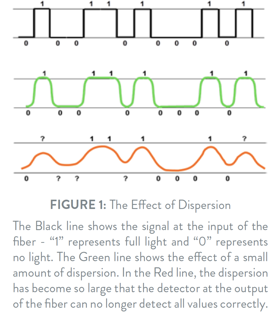
Much, but not all, of the traffic traveling through fiber networks takes the form of pulses of laser light. Such a pulse is created by turning a laser on and off, creating light pulses where “no light” represents a digital “0” – and “full light” represents a digital “1”. Digital information is consequently a series of “no light” and “full light” transmitted in a code which a receiver at the other end of the fiber understands and can convert to a digital electrical signal.
Illustrating such a signal would be a series of square pulses as shown in Figure 1.
Whenever such a signal is affected by dispersion, the edges of the square pulses will be rounded, and the pulse will be spread out over time. So dispersion broadens the pulses.
If the dispersion is small, the detector at the other end of the fiber will still be able to detect the signal correctly. Once the dispersion grows too large, the broadened pulses will overlap each other and the detector will start misreading the signal, creating errors that will effectively hamper the transmission quality. A measure of that quality is the BER (Bit Error Rate) which states the number of transmission errors relative to the total number of transmitted bits.
Since a faster transmission rate requires pulses to be of a shorter duration, this also means that a given level of dispersion will be more harmful to faster transmission rate signals. Furthermore, dispersion is almost always dependent on the fiber length – the longer the fiber, the greater the dispersion.
Hence transmission is limited by: A) The dispersion of the fiber B) The transmission rate, and C) The length of the fiber. Dispersion can be described as a “speed limiter”- and the 3 main types are:
Modal Dispersion, Chromatic Dispersion and Polarization Mode Dispersion.
Modal Dispersion is the most serious of the dispersion types, and hence the most severe “speed limiter”.
Light “modes” are different types of waves carrying the light through the fiber. In a “Multi Mode” fiber, the core is rather large and may typically allow up to 17 different modes to propagate. In a “Single Mode” fiber, the core is so small that it will allow only one mode to propagate.
The problem is that the different modes follow different paths through the fiber – and these paths are of different lengths. Some modes travel close to the center of the core – others bounce against the outer edges of the core, and these modes travel a longer way than the ones close to the center. So the different modes travel different distances – and hence some tend to travel faster than others. Parts of the light being injected into the fiber will travel via one mode – other parts via another mode – and so on. If nothing is done to mitigate this, parts of the input signal will arrive at the output later than other parts – and this will cause the output signal to be “dispersed” relative to the input signal as illustrated in Figure 1.
To try to minimize the dispersion of the signal to the output of the fiber, the fiber core of a multimode fiber is designed to delay the Light Modes travelling close to the core (which is the shortest distance) and to speed up the modes travelling the longest distance. In a perfect world this would result in all modes bringing light simultaneously to the output of the fiber. Alas the world is less than perfect, and as such a bit of Modal Dispersion cannot be avoided in real life.
This means that, even though Multimode fibers are able to use very price efficient light sources (like LEDs or VCSELs) they are still limited to transmission distances of typically less than 2 km, actually often less than a few hundred meters.
The way to avoid Modal Dispersion is to shrink the size of the fiber core. In a small fiber core there is only room for one light mode to exist, called the Fundamental Mode. In such single-mode fibers, higher order modes may indeed be generated at splices or connectors, but they will leak out of the fiber after traveling a short distance through the fiber.
Having now found a way to avoid the most important speed limiter we can turn our attention to the next in line.
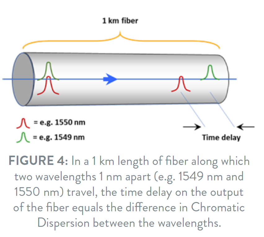
Chromatic Dispersion means that light of different wavelengths travel with different speeds along the fiber. Again, such a difference results in the “blurring” of the signal on the output side of the fiber and effectively acts as a speed limiter.
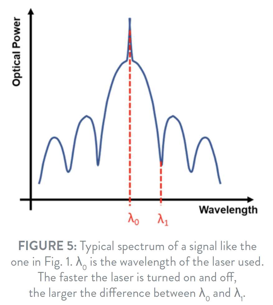
One might wonder why this should be such a problem, since lasers used to inject light into the fiber have very precisely defined and stable wavelengths. However, quickly turning a laser light on and off actually by itself generates a number of new wavelengths close to the original laser wavelength. Most of these new wavelengths are luckily quite weak and will not cause problems – but unfortunately as the laser light is turned on and off ever more quickly, the range of generated wavelengths broadens (Figure 5).
In such transmission systems the problems caused by Chromatic Dispersion worsen with increasing transmission speed and with longer fiber lengths (scaling linearly with fiber length).
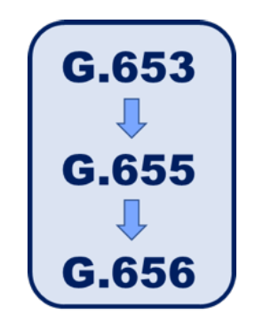
Trying to minimize problems with Chromatic Dispersion the “Dispersion Shifted” (ITU-T G.653) fiber type was initially developed. In classical standard single-mode (ITU-T G.652) fibers the Chromatic Dispersion is zero around 1310 nm. The Dispersion Shifted fibers were targeted for the Chromatic Dispersion to be zero around 1550 nm, because the attenuation of the fiber is lower at 1550 nm and so this combination seemed ideal.
Basically, this worked fine right up until DWDM arrived. In DWDM systems a number of individual channels are transmitted over the same fiber. Each channel is assigned a unique wavelength, but unfortunately the fiber non-linearity called Four Wave Mixing (FWM) tends to cause unwanted noise problems in DWDM systems if the Chromatic Dispersion in the fiber is very low.
So realizing that some level of Chromatic Dispersion is preferable in order to limit fiber non-linearity problems in DWDM systems, Non-Zero Dispersion Shifted fiber (ITU-T G.655) was developed. This fiber type has a small amount of Chromatic Dispersion around 1550 nm (significantly smaller than standard G.652 fibers) so the “speed limitation” is smaller – but still the Chromatic Dispersion is high enough to reduce non-linearity problems very significantly. Later the G.656 Non- Zero Dispersion Shifted fibers were developed as a response to the demand for an increasing number of channels in DWDM systems. When the number of channels go up, the individual channels need to be packed more closely together – and that in turn requires more Chromatic Dispersion in the fiber to reduce the effect of the Four Wave Mixing.
In parallel with the development of new fiber types with different Chromatic Dispersion characteristics, special devices with negative Chromatic Dispersion were developed. Since transmission fibers normally have positive Chromatic Dispersion, a combination of those two can be used to reduce total Chromatic Dispersion for a full fiber link to almost zero.
With the ability to reduce the total chromatic dispersion of a transmission link, the higher Chromatic Dispersion of the G.656 fibers was consequently an acceptable technical compromise – leaving only cost issues still to be considered.
In many of the recent high-capacity transmission systems, the Chromatic Dispersion of the transmission fiber is compensated electronically with high efficiency, and for such systems fibers with high Chromatic Dispersion may actually be advantageous because it helps to limit fiber non-linearities.
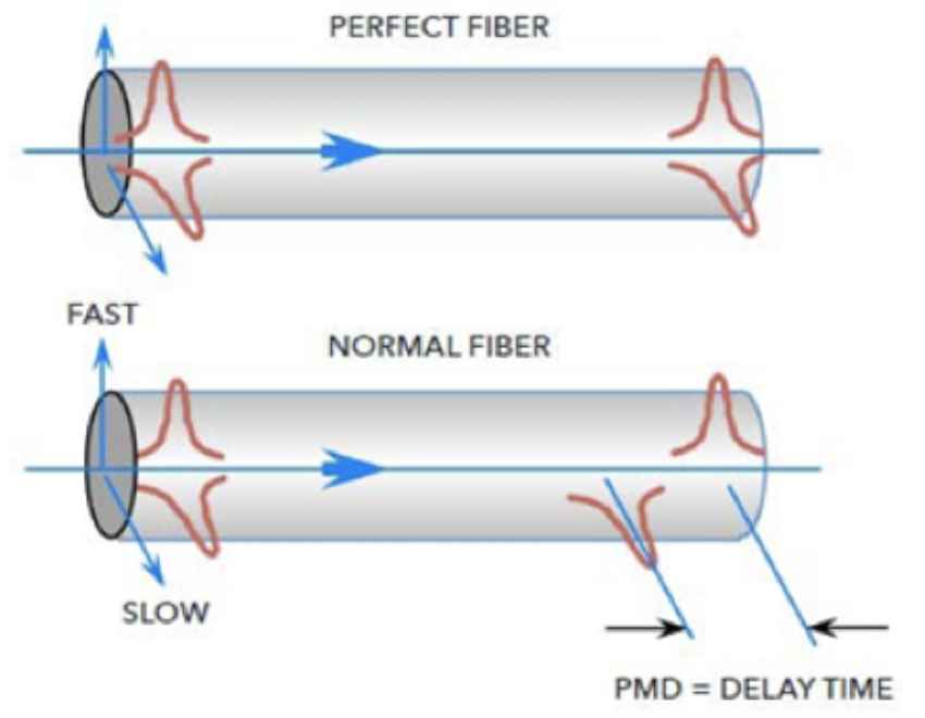
Just to make confusion complete, a single-mode fiber will actually be able to carry TWO versions of the fundamental light mode. The reason for this is that light may exist in two different polarizations, the modes of which are perpendicular to one another. The phenomenon is known from some sunglasses which cut away one of those polarization modes. Reflected sunlight from the sea surface or a wet road will predominantly consist of light in one of these polarization modes – whereas light reflected by other objects will consist of a mixture of the two polarization modes. Cutting away the polarization mode of the reflected light will “kill” the reflections, but let the other polarization mode pass through the glasses, leaving other objects visible.
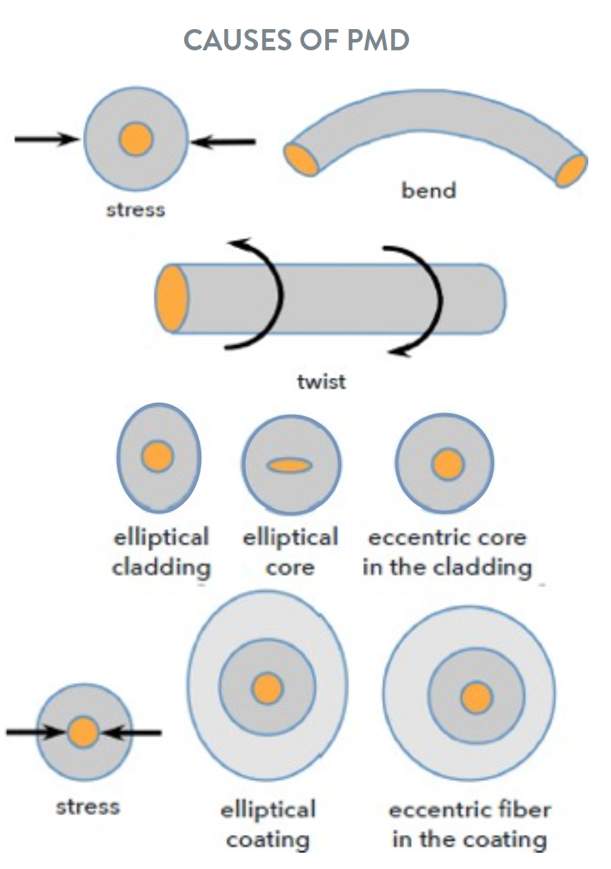
In an optical fiber, the two polarization modes will both exist, but may travel at different speeds through the fiber. Such speed-differences will arise if the fiber core is not perfectly circular and if stress is present in the fiber. Stress can be “frozen” into the fiber during manufacturing if the fiber geometry is not absolutely perfect, for example, if the cladding or coating is not circular, or if the center of the core is different from the center of the cladding or coating.
Even using state of the art, high-quality manufacturing process, the fiber will not be geometrically 100% perfect, hence there will be a speed-difference between the two polarization modes, dispersion will result, and it may limit high speed transmission through the fiber. Even if the fiber were 100% perfect, the slight bending of the fiber in a cable would introduce stress in the fiber – creating PMD. So this is our third speed limiter.
Looking at a fiber from a “PMD-perspective” it may be thought of as having a “fast” and a “slow” lane. An effective way of reducing PMD is by twisting the fiber back and forth during manufacturing so that a high number of shifts between the “fast” and “slow” lanes are effectively seen by the light travelling through the fiber.
Because stress is an important cause of PMD, externally applied stress will also affect fiber PMD. In reality just holding a fiber between two fingers may change PMD. As a result, the PMD of a fiber may be affected both by the cabling of the fiber and by external stresses, for example vibrations from a nearby railroad.
As with other dispersion types the effect of PMD increases with increased transmission distance (PMD scales with the square root of the distance) and increased transmission speed. For transmission rates of 2.5 Gbps and smaller, PMD is normally not a problem. For very high transmission rate systems, the compensation of PMD is today made electronically and built into the transmission system.
The fiber optic cable world has come a long way over the past 30 years. Products have become more rugged and user friendly, making it easier for people to enter the industry and work handling optical fiber and cable. While this is great for the industry, many people may understand the “how to” but not necessarily the “why” of fiber optics. To understand the “why” behind fiber and cable products, the next step is to become a full-fledged “fiber geek.” Because the industry changes so quickly, this is an ongoing process. The purpose behind this series of articles is to enable the reader to understand some secondary fiber specifications and their importance to the network.
Once fiber is deployed, it’s very expensive to replace. For this reason, the fiber that’s installed should be capable of withstanding multiple generations of hardware while also having plenty of room for additional wavelength growth.
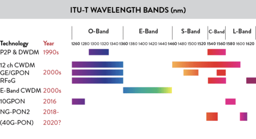
FIGURE 1: Already Defined ITU-T Wavelength Band
The graphic on the right highlights how wavelength usage has grown over the past three decades. For the first 30 years, applications were focused in the 1310 nm and 1550 nm regions. Given the explosive demand for bandwidth (even more so since COVID-19), it’s reasonable to assume that the next 30 years will require many more wavelengths, with potential applications across the entire optical spectrum.
The demand for bandwidth is expected to continue far into the future, driven in part by requirements for breakthrough applications such as higher resolution video, virtual reality and other applications. We expect this demand to continue to drive the need for optical spectrum provided by fiber. Fiber recommendations such as ITU-T G.652 and ITU-T G.657, are very important for network designers in setting minimum performance levels, but can ultimately be insufficient to meet the requirements for future networks. For this reason, performance beyond the standards can be very important.
This article will focus on critical optical parameters starting with attenuation, or loss in the fiber. Attenuation is a very important optical parameter, and there are many aspects to it. Additional articles in this series will focus on other optical parameters, including chromatic and polarization mode dispersion, splice loss, and an introduction to non-linear effects.
Keeping a low fiber attenuation has always been a focal point in fiber development – and today even more so with the widespread use of Coherent Transmission systems. These require large core and ultra-low loss attenuation fibers (typically ITU-T G.654 fiber types) for optimal performance of 100G and faster transmission systems.
Attenuation is typically measured in terms of optical dB. It is a logarithmic measurement where the Loss of a fiber equals 10*log (“Power at the- input side of the fiber” / “Power at the output side of the fiber”). Basically every 3 dB of loss corresponds to the optical power being cut in half. It is fair to assume, that the attenuation of a fiber is almost constant over the length of the fiber. So if a fiber loss is 0.25 dB/km, a total loss of 3 dB will be reached after 12 km of fiber has been passed by the optical signal in the fiber.
Looking at the different loss mechanisms in fibers, it may be helpful to distinguish between:
A): Attenuation caused by factors external to the fiber (as for example bending), and
B): Built in attenuation mechanisms.
Looking at B) first, there are two main loss mechanisms in optical fibers: Scattering and Absorption.
SCATTERING
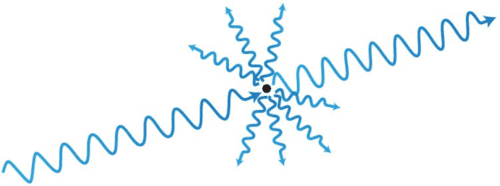
FIGURE 2: Scattering of Light in All Directions
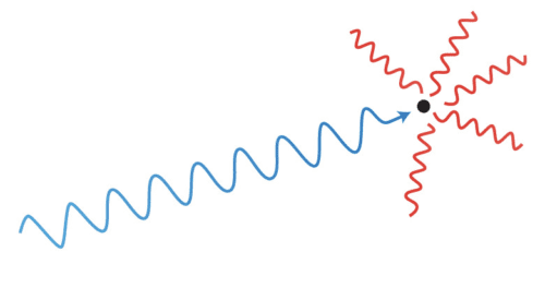
Also called “Rayleigh scattering”, even the best and purest, synthetic quartz glass (of which OFS fibers are made) is not 100% homogeneous. They consequently contain small fluctuations of glass density, which are frozen into the glass during manufacturing and may scatter the light when hit by a light ray (this is the same mechanism responsible for the blue color of the sky, when sunlight scatters off molecules in the atmosphere). Much of the light will continue traveling in the original direction, but a small part of the light will be scattered in all directions. Some light will propagate sideways out of the fiber, where – for transmission purposes – it will be lost. Some of it will actually be scattered backwards towards the sender. This is the phenomenon used by OTDR measurement devices to measure fiber attenuation, so the device only needs to be connected to one end of the fiber.
In optical fibers scattering is dominant at shorter wavelengths whereas the opposite is true for the other built in attenuation mechanism: Absorption (Figure 4).
ABSORPTION
FIGURE 3: Absorption, Light Converted to Heat
Basically absorption happens when a light ray hits something – and gets converted into heat. So for practical purposes the light simply “disappears”.
Even extremely small impurities – down to a fraction of a micron – may absorb light, causing unwanted attenuation. It may be small particles – but it may also be impurities in the raw materials used for fiber manufacturing. This is why such extremely close attention is paid to the quality and purity of the raw materials used.
Due to the inherent material structure of glass, Absorption increases rather drastically at wavelengths longer than approximately 1550 nm (Figure 4)
Of particular interest over the years has been the hydroxyl (OH-) ion, which absorbs light around 1383 nm, giving rise to the so-called “water-peak” in the attenuation curve for the fiber (figure 5 – black curve). Being a by-product of the actual manufacturing process, it is difficult to fully avoid the presence of hydroxyl ions in the fiber, but it is possible to pacify the attenuation increase at the wavelengths close to 1383 nm. This is done by adding deuterium gas which interacts with the free bond of the hydroxyl ion thereby acting as a barrier securing excellent long-term Water Peak attenuation performance.
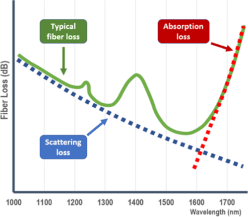
FIGURE 4: Scattering and Absorption Wavelength Dependency
Conventional single-mode fibers meeting the G.652 recommendation may have a high Water Peak loss. This could limit the use of the fiber in some applications and may also make the fiber less useful in transmission systems using modern Raman amplification, where amplifier laser-pumps would typically operate 110 nm below the transmission signal wavelength.
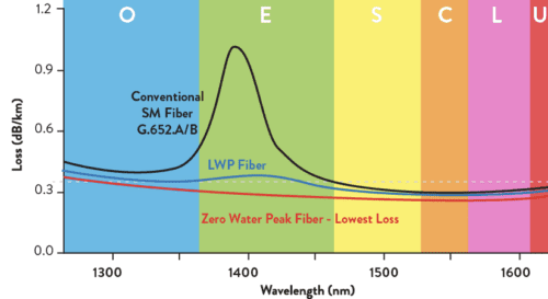
OFS have fibers classified as Zero Water Peak (ZWP) with even better specified Water Peak performance than the so-called Low Water Peak (LWP) fibers. The long-term stability of ZWP fibers is excellent whereas for some types of ITU-T G.652 fibers the water peak attenuation might actually increase over their lifetime, slowly reducing the quality of the network.
Because of the optimized Water Peak performance, ZWP fibers serve the widest ranges of wavelengths and support the highest number of applications, as illustrated in Figure 1.
Figure 5 shows three different grades of ITU-T G.652 fiber, and how they may be performing in the water peak region around 1383 nm.
FIGURE 5: Water Peak Loss of Three Fiber Grades
For the most part, scattering and absorption properties are locked into the fiber during manufacturing.
Bending, however, is another story…
BENDING
Bending is a very important mechanism. As briefly mentioned, it is caused by factors external to the fiber and so both the cabling process and installation in the field can affect attenuation caused by bending.
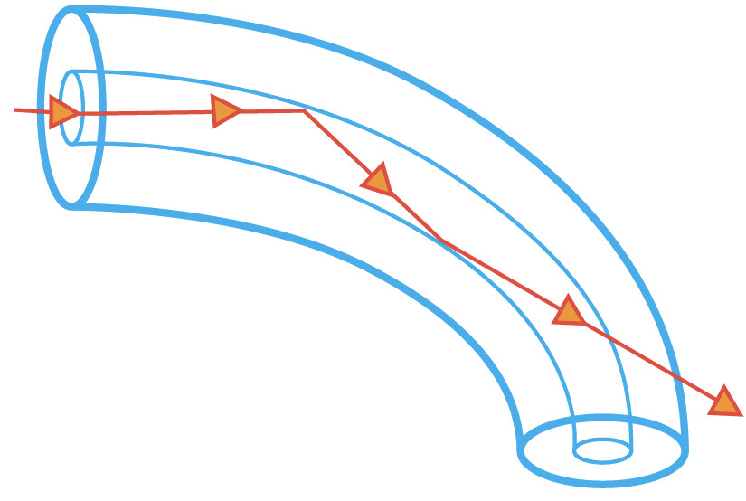
FIGURE 6: Macrobending Light will leak out of tight bends.
To put it simply, what makes an optical fiber work is the use of different types of glass for the fiber core and for the glass surrounding the core (also known as the cladding). In this way, a sort of a tubular mirror surrounding the core is created. This is what keeps the light inside the fiber, using the concept of “total internal reflection” to guide the light. However, this mirror is not a perfect one. It only works if the light rays in the fiber run almost parallel to the core, and so if the fiber is bent (too) tightly (i.e. past the “critical angle” when reflection turns to refraction), light will leak out of the fiber causing loss – or attenuation.
This is called macro bending, where the diameter of the bending is larger than a few millimeters, which is what one would intuitively understand as “bending” the fiber.
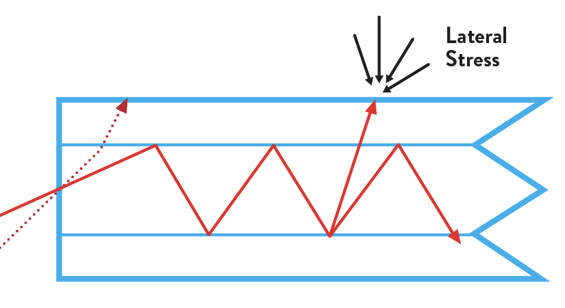
FIGURE 7: Microbending Loss caused by lateral stress.
Another type of bending is called micro bending. It concerns bending diameters smaller than 1 mm and could happen – as an example – if a fiber is squeezed between two sheets of sandpaper. Much more relevantly it may also happen if the fiber is being squeezed inside the cable construction (for example by the tubes containing the fibers) creating stress on the fiber. As loads/stresses increase, so does the loss.
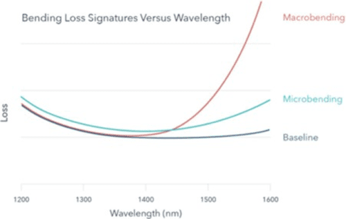
Both types of bending loss cause attenuation increase, but it is possible to tell the two types of bending apart by considering the added loss at different wavelengths as illustrated in Figure 8.
Macrobending losses tend to be small at short wavelengths, but may increase rather dramatically at longer wavelengths.
FIGURE 8: Difference between Micro-and Macro-Bending Loss vs. Wavelength
Microbending losses are also typically present at short wavelengths, but the loss increase tends to be smaller than for macrobending at the longer wavelengths.
All of the trends in fiber deployment point to the increased importance of fiber bending performance.
Service providers constantly want to put more fibers into a smaller space which means that while buffer tube diameters keep shrinking, the fiber counts used in these buffer tubes keep increasing. This leads to a situation where there is less room for fibers to move before touching a buffer tube wall, thereby increasing the risk of microbends.
In addition, service providers primarily installed cables in either the outside plant, the inside of central offices, or into remote cabinets. Everywhere great care was taken to avoid small diameter bending. However, today’s fiber is going to places where it hasn’t gone before. It’s going inside our homes and businesses and also up poles and onto rooftops to feed cellular and Wi-Fi sites.
Tolerance to bending will be even more important in the future.
Micro and macro bends affect the network in ways that are not always obvious.
Bend-related losses are sometimes experienced in cold temperature environments. For this reason, fibers and cables should always be tested under low temperature conditions. As a network designer, it’s always a good idea to account for at least some optical margin for small potential attenuation increases in cold temperatures.
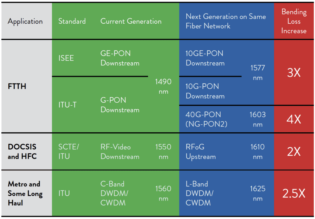
FIGURE 9: Next Generation Fiber Networks may use longer wavelengths than today – increasing requirements for low bending
loss fibers already now.
Especially very high-density designs may benefit from using bend insensitive fibers due to the unavoidable bends and lack of free space for fiber movement in the cable design itself.
While these issues are already important today, they will become even more important tomorrow. The reason is that next generation optical transmission protocols may typically use longer wavelengths than the existing protocols.
As highlighted earlier, longer wavelengths will often result in higher bending loss. Theoretically, a GPON network operating flawlessly today at 1490 nm – containing inadvertent bends – could have its reach reduced by almost half when it is upgraded to NG-PON2, operating at 1603 nm.
So a FTTH network installed today and working fine may not be suited for operation with future generation transmission equipment.
HELP IS ON THE WAY
In order to enable more compact cable constructions and allow for easier installation and perhaps even allow for the use of less experienced craftspeople for cable installation, quite a bit of attention has recently been focused on developing fibers with reduced sensitivity to bending i.e. those defined by the ITU-T Recommendation G.657.
G.657 specifies 4 different classes of fibers: “A1”, “A2”, “B2” and “B3”.
The “A” fibers are required to also fulfill (or to comply with) the specifications of the ITU-T G.652.D recommendation, whereas the “B” fibers may deviate from G.652.D on some parameters. The numbers (1, 2 or 3) signifies the fibers tolerance to bending – B3 fibers being most bending tolerant. Many “B3” fibers do today comply with G.652.D and should rightfully be labelled: “A3”, but such a class is not specified by ITU-T.
ITU-T G.657.A1 fibers are the closest to standard G.652.D fibers and may soon be the primary choice for the vast majority of fiber networks. OFS has combined G.657. A1 and G.652.D performance with a 9.2-micron mode field diameter.
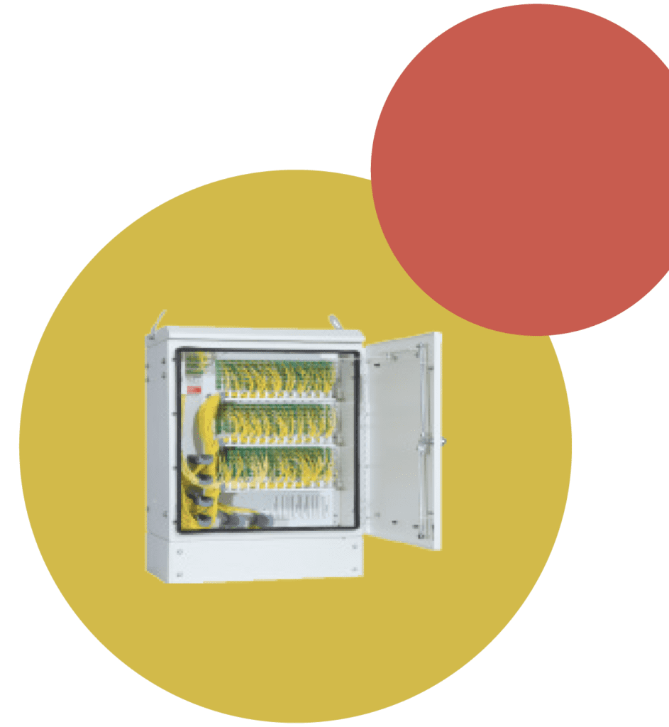
FIGURE 10: Fiber Distribution Hub
G.657.A1 fibers with 9.2-micron mode field diameter perform the same way as standard G.652 fibers in terms of splicing – and can consequently be said to splice “seamlessly” to the huge base of already installed fibers. By offering the same splice performance as standard G.652 fibers, installation crews and quality inspectors will notice no change in performance and hence be given no cause for concern – even
though the advantages of better tolerance to bending will still be there.
These fibers are ideal for most of today’s typical short-distance (<1000 km) and low data rate (<400Gbps) applications, including standard outside plant (OSP) loose tube, ribbon, rollable ribbon, microduct cables, and drop cables.
ITU-T G.657.A2 fibers can be bent more tightly with lower loss. They are most commonly used in central office and cabinet environments, such as Fiber Distribution Hubs (FDH). These fibers are also commonly used in building backbone networks and as tails for various pre-terminated panels and other devices. In these environments, the fibers may need to be bent more tightly than in typical OSP cable applications.
The application spaces just mentioned for A1 and A2 fibers would typically involve one fiber to carry traffic for thousands of customers, meaning that a fiber break would affect the service to thousands of users. Here reliability is consequently paramount. In such situations A2 fibers (and A1 as well) offer the advantage of providing an “early warning” signal of increased attenuation whenever they are bent tightly enough to potentially cause reliability concerns. This is especially important for central office applications where one fiber could provide the feed for millions of customers.
ITU-T G.657.B3 fibers are the third main category of bend insensitive fibers. These fibers are designed and recommended for use in the drop portion of a Fiber-to-the- Home (FTTH) network serving a few customers per fiber. Homes and buildings with lots of tight spaces are very demanding places to deploy fiber. For optimized performance in such applications OFS has fiber which is designed and specified for use with bending radii as low as 2.5 mm which is significantly less than the minimum bending radius of 5 mm specified in the G.657.B3 recommendation.
OFS has fibers used in cables with a diameter of only 0.6 mm, enabling almost invisible in-house cable routing with a minimum of bending management. This avoids bulky and distasteful installation in private homes. For more demanding deployments, ruggedized cable designs with a diameter of 4.8 or 3mm may even be routed around corners and stapled using fast and easy installation practices, with negligible signal loss.
G.657 fibers which are not compliant with G.652.D are often assumed to have very small cores giving rise to significant additional splice losses when spliced to standard G.652.D fibers. However, that is not necessarily so. It is possible to get G.657.B3 fibers specified with an ultra-low bending radii of 2.5 mm and – whereas these fibers are not “seamless” fibers – they do in fact comply with the G.652.D recommendation in terms of core size. The only thing preventing such fibers from complying with G.652.D is the Chromatic Dispersion, and since they are primarily intended for in-building applications, the length will typically be much less than the 10 – 40 km fiber length in which the higher Chromatic Dispersion may typically start presenting problems.
Regarding bending loss however, the performance of such a fiber is significantly better. The loss for a single turn of 2.5 mm radius at 1550 nm for such a fiber is max. 0.2 dB – whereas the similar loss for a standard G.652.D fiber exceeds 30 dB.
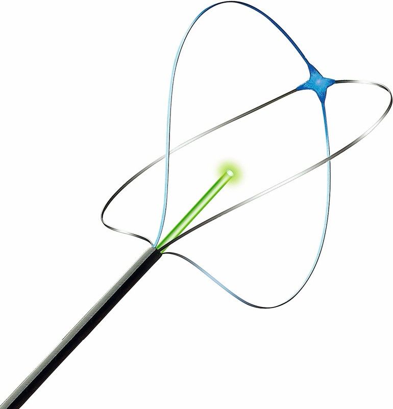
A German manufacturer of stone-retrieval baskets works with a U.S. manufacturer of specialty optical fiber. The result is a basket that, thanks to its coaxially integrated optical fiber, can simplify and shorten minimally invasive urological surgery.
The treatment of kidney stones has changed dramatically over the years. Instead of open surgery, today minimally invasive endoscopic-based procedures can be used. Once a stone is found, it can usually be removed using a nitinol basket. If the stone is too far up the urinary tract, fragmentation using laser energy is used to pulverize it. Pulverization is achieved by the introduction of an optical fiber to deliver the laser energy. This procedure is called intracorporeal lithotripsy.
Pulverization using laser energy may vary. Combining a long pulse duration with low pulse energy and high pulse frequency will blast the stone into dust. The small dust particles are eliminated, naturally. But the high pulse energy will cause the ambient temperature to rise and may cause damage to surrounding tissue. An alternative to pulverization is fragmentation. Fragmentation uses laser energy with a short pulse duration, high pulse energy and low pulse frequency. The resulting fragments can then be captured using a stone-retrieval basket.
Usually the stone is fragmented prior to the pieces being captured by the basket. But sometimes, depending on the location of the stone, the reverse order is necessary. In these cases, where the stone is captured and then fragmented, there is the risk of the laser energy damaging the stone-retrieval basket as well as the surrounding tissue.
The next logical development in intracorporeal lithotripsy is an instrument that coaxially integrates optical fiber with the stone-retrieval basket. This improved instrument enables positioning of the basked and the optical fiber at the same time. The stone is safely trapped and fragmented without damaging surrounding tissue or the basket. Surgery time is shortened since only one instrument is needed.
This new device was developed by Endosmart GmbH in Stutensee, Germany together with OFS, a U.S. designer and manufacturer of specialty optical fiber.
A typical laser system for lithotripsy is based on Ho:YAG (Holmium:Yttrium-Aluminum-Garnet) laser which uses at a wavelength of 2123 nm with an average power of 30 W. Pulse duration, peak power and frequency are adjusted according to the individual treatment. For example, the laser pulse could be up to 18 kW peak power or 3.5 J pulse energy. To enable orientation of the instrument, the system delivers a visible red or green pilot light.
Light is guided even under extreme bending
The step-index multimode optical fiber used to guide the laser can have a pure silica core and a fluorine-doped glass cladding or a Germanium-doped core with a pure silica cladding. The different refractive indices of core and cladding enable the laser to propagate longitudinally in the fiber core. For guiding the light under extreme bending, an additional UV cured fluoroacrylate coating is applied. The fluoroacrylate coating has a lower refractive index than either of the glass claddings and acts as a secondary cladding for guiding the light. The optical fiber that is used with the nitinol basket described above has a core diameter of 272 µm and a silica cladding diameter of 299 µm. Around that, a 330 µm UV cured fluoropolymer coating is applied acting as a second optical cladding and finally, an ETFE buffer of 400 µm is applied.
Glass fibers are also used for medical diagnostics. Current developments are focused on simultaneous diagnosis and treatment.
In today’s increasingly fast-paced, interconnected world, the need for high-speed broadband internet access and reliable wireless service is more acute than ever. The growth of fiber optic networks has allowed service providers to optimize FTTx — fiber-to-the-X, in which X can refer to various subscriber locations, including homes (H, as in FTTH) and buildings (B, as in FTTB) — with the most effective, cost-efficient connectivity and bandwidth capabilities.
Optical fiber solutions guarantee subscribers high-quality transmission of video, voice, and data while providing comprehensive end-to-end solutions for maximum return on investment (ROI). Fiber optics also allow subscribers to make use of recreational technologies such as HDTV, video on demand, and online gaming.
To reach and connect subscribers InvisiLight® Solutions, feature solid glass optical fiber bendable down to a 2.5-mm radius with practically zero loss. This innovative and patented technology provides a 500-fold improvement in bending loss over traditional approaches that use Single-Mode Fiber (SMF) type cables. The flexibility of this solution simplifies and hides installations by conforming to building corners, with no concern for bending loss or service disruptions.
WhatInvisiLight Indoor Living Unit (ILU) Solution Do I Need?
The OFS InvisiLight ILU Solution guide can help you decide which of the four InvisiLight ILU Solutions to use, based on your needs. Whether you are looking for low visibility, low cost, greater security, or ethernet connection for business we have the answer for you.
InvisiLight Indoor Living Unit (ILU) Solution Guide
History
Launched in 2012, the original, award-winning InvisiLight ILU Solution offered installers an innovative and simple method for indoor optical fiber installation. Since then we have launched added variations that are adaptable depending on customer needs. The process involves adhering a 0.9 mm diameter optical fiber into either crevices along ceilings and walls or moldings and walls. The result is a protected optical fiber link that is virtually invisible.
Very EZ
All InvisiLight products feature innovative OFS EZ-Bend® Optical Fiber. This fiber’s 2.5 mm minimum bend radius easily handles the sharp corners often met when installers conform optical fiber to a building.
When you are ready to order, or require more information, our experts are standing by ready to help. Simply fill out the form here.


 In today’s increasingly fast-paced, interconnected world, the need for high-speed broadband internet access and reliable wireless service is more acute than ever. The growth of fiber optic networks has allowed service providers to optimize