
WELCOME BACK, FIBER GEEKS!
The first Article in this series focused on growth in bandwidth demand and attenuation in optical fibers. Article 2 concentrated on the several types of dispersion that exist in fiber today, closely followed by Article 3 – Fiber strength and reliability. Article 4 featured single-mode fiber geometries and now the latest release from OFS – Article 5, deals with “Cut-off Wavelength” (COW). This latest article will help the user to understand what “cut-off wavelength” is, why does it matter and how is it measured.
CUT-OFF WAVELENGTH MAKES A COMEBACK IN IMPORTANCE
Take an intro to fiber course, and you’ll learn about attenuation, dispersion, fiber geometry, maybe fiber strength. However, buried in the fine print of fiber specs is a parameter called cutoff wavelength. Although fiber manufacturers and some fiber users are aware of cutoff wavelength, it’s not as famous a parameter. Users still focus primarily on attenuation, maybe dispersion, as critical propagation properties.
Due to relatively new operating wavelength requirements below 1310 nm, some astute end users are taking a renewed look at cutoff wavelength specifications. Relatively new Passive Optical Network (PON) protocols are looking at wavelengths as low as 1270 nm, which, optical spectrum-speaking, is a hop and a jump away from the historical cable cutoff wavelength specification λcc, 1260 nm.
Different fibers do different jobs in today’s networks. Some fibers are bend insensitive. Some fibers enable more power to increase signal-to-noise ratios at ultra-high speeds. Cutoff wavelength is important for the performance of these fibers, but these fibers may require differences in measurement methods versus “standard” G.652-type fibers. We’ll talk about measurement methods later in this paper.
WHAT IS CUT-OFF WAVELENGTH?
In an optical fiber a number of different light-“modes” may exist. Modes are different types of light waves which may each carry different portions of light from the input to the output of the fiber.
A multimode fiber, by definition, may carry several modes of light (several hundred), but in a single-mode fiber, only one mode is carried.
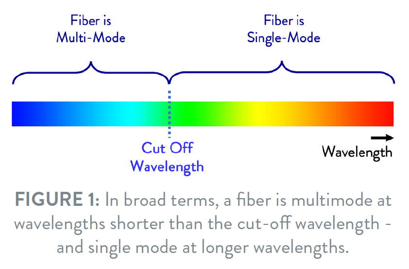
The wavelength at which the fiber is at the cusp of changing from single-mode to multi-mode is called the Cut-off Wavelength. Typically, a fiber is considered to be single mode for wavelengths longer than the Cut-off Wavelength (COW) – and multimode at shorter wavelengths. In real life, the transition from single mode to multi-mode transmission does not occur abruptly at an isolated wavelength – but rather relatively smoothly over a range of wavelengths. The single-wavelength number on a specification is a simplification.
The most common way to make a fiber single-mode is to reduce its core-size (diameter), but the contrast between the refractive index of the fiber core and the fiber cladding is also important. These two properties determine the “effective core size” which determines if the fiber is single mode or not at a given wavelength.
WHY IS IT IMPORTANT?
The whole idea of a single-mode fiber is to keep the other modes out of the optical transmission. The reason is why Multi-Mode fibers are used for short distance transmission only: different modes traveling through a fiber take different paths.
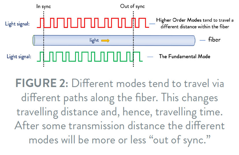
An optical pulse injected into a multi-mode fiber will be transmitted via different modes reaching the end of the fiber after slightly different travel times. Once the modes are recombined at the output of the fiber, the shape of the input pulse will have been distorted (blurred). This distorting effect on the pulse is known as modal dispersion and affects the bandwidth (MHz-km) of a multimode fiber. Single-mode fiber does not have modal dispersion, and consequently has much higher bandwidth over dramatically longer distances.
The concept of cutoff wavelength is receiving renewed attention as next generation PON systems begin operating at wavelengths shorter than 1310 nm. This will be discussed in more depth later in the paper.
“ONLY ONE LIGHT MODE IN MY SINGLE MODE FIBER, PLEASE!”
The light mode intended for transmission in a single mode fiber is called the Fundamental Mode (also called LP01). All other modes are called Higher Order Modes, the most important of those is the Secondary Mode (LP11).
And one might ask: “Where do those higher order modes come from?”
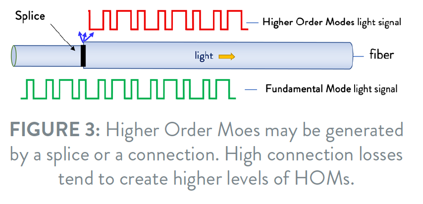
These modes may be generated at splices and connections between fibers. The higher the splice/connection loss, the more powerful the Higher Order Modes (HOM) tend to be generated.
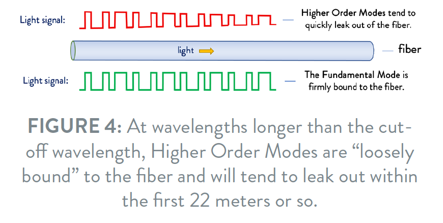
HOMs are also called “leaky modes” because they are bound only loosely to the fiber core and tend to leak out of the fiber after traveling a relatively short distance – for wavelengths longer than the Cut-off Wavelength. The longer the distance, the more of those modes will have leaked out.
The Cut-off Wavelength is defined as the wavelength at which the power level of the Higher Order Modes has been reduced by 19.3 dB relative to the level of the Fundamental Mode (strictly speaking this is true only for the Second Order Mode).
MODAL NOISE PROBLEMS
Do we need to worry about modal noise in today’s systems? Without wanting to raise unwarranted concerns, we want to highlight possible situations where modal noise may arise and be problematic.
As briefly mentioned, splices or connectors will cause some of the light in the Fundamental Mode to be coupled into higher order modes. And likewise, light from Higher Order light modes may be coupled down into the fundamental mode by similar splices or connectors.
Situations may arise where two splices or connectors are situated closely to each other. If they are too close, or if the Cut-off Wavelength is too high, parts of the HOMs generated at the first splice/connector may be coupled back down into the Fundamental Mode at the second splice/connector and mixed with light from the initial Fundamental Mode.
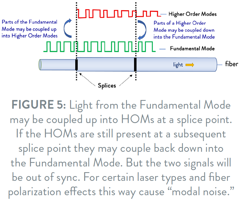
This may cause a problem because the travelling time for the light signal may typically be different in the Higher Order Modes than in the Fundamental Mode – and so the two signals may be somewhat out of phase when mixed together. Because of polarization and other effects, such phase difference may change as a result of temperature variation and stress, and this can result in a type of noise called Modal Noise.
To create significant levels of modal noise two joints with large connection losses must exist (one is not enough). Furthermore, the two joints must be so closely spaced that Higher Order Modes have not leaked out of the fiber before reaching the second joint. And finally, the laser used must exhibit some level of mode partitioning.
WHY ARE THERE DIFFERENT TYPES OF CUT-OFF WAVELENGTH?
The Cut-off Wavelength of a fiber depends on the length of the fiber, the longer the fiber the lower the Cut-off Wavelength tends to be. For that reason, there are 3 types of Cut-off Wavelengths defined to match different applications:
- CABLE CUT-OFF WAVELENGTH (λcc): It is very easy to mistake this term for “Cabled COW” – but in principle it does not really matter whether the fiber is cabled or not. The initial intention with this parameter was to simulate a situation with two closely spaced cable splices, for example in a repair situation. 20 meters splicing distance was considered a relevant minimum – and to simulate fiber being deployed in splice cassettes, a 1-meter fiber length including one 80 mm loop was added in each end for the measurement set up. Effectively the full length of the fiber measured is 22 meters.
- JUMPER CUT-OFF WAVELENGTH (λcj): As the name suggests it simulates a jumper cable. It is measured on a 2-meter length of fiber with one winding which diameter may be freely defined – which in the US is typically 152 mm.
- FIBER CUT-OFF WAVELENGTH (λcf): As the name suggests it simulates a fiber being bent in only large diameters. In principle it is measured on a 2-meter length of fiber with one 280 mm diameter, but as explained later special care must be taken during measuring – especially for bend-insensitive fibers.
Because Cable COW is measured on a 22 m fiber sample whereas Fiber COW is measured on 2 m fiber, Fiber COW is typically higher than Cable COW.
Normally it is possible to find a good statistical correlation between the Cable COW and the Fiber COW. Since only 2-meter fiber is needed when measuring Fiber COW, it is easier to measure Fiber COW than Cable COW where 22 meters are needed. And because of the correlation Fiber COW measurements are often sufficient to ensure that the Cable COW is within limits.
Also, cabling fibers often has an effect of stripping out higher order modes, due to either macro or micro-bending of the fibers inside the cable sheath. In situations where this effect is significant, Cable COW measured on a cabled fiber may be lower than Cable COW measured on a non-cabled fiber (and of course lower than Fiber COW).
It depends on the fiber type and design, but a realistic example for a step-index fiber is a fiber cutoff of 1350 nm could have a corresponding cable COW of 1260 nm.
WHY IS CABLE CUT-OFF WAVELENGTH SPECIFIED AS 1260 nm IN IEC AND ITU-T RECOMMENDATIONS?
Initially Single Mode fibers were intended for 1310 nm operation, and manufacturing variability of lasers were rather large, so lasers sold as “1310 nm lasers” could in fact emit light at rather different wavelengths than 1310 nm. So, to create a certain “guard band”, the maximum Cable COW was defined to be 1260 nm.
Today, laser wavelengths may be more tightly controlled and extremely accurate, but those lasers may also be more costly than less accurate lasers. Furthermore, some FTTH/PON transmission formats (especially newer ones such as XGS-PON) use wavelengths close to 1260 nm. So, the 1260 nm COW today has renewed relevance.
BEND-INSENSITIVE FIBERS – AND PROBLEMS MEASURING THEIR ATTENUATION
This may seem like a subject entirely different from Cut-off Wavelength – but measurement problems are quite similar and may not be obvious at all.
To determine the Cut-off Wavelength, two measurements of the power on the output of the fiber are compared:
A. Power in the Fundamental Mode (LP01) only
B. Power in the Fundamental Mode (LP01) and the Higher Order Modes (which in practical terms means the Second Order Mode: LP11)
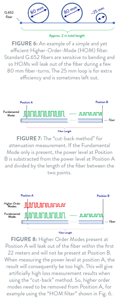
“B” is just a simple measurement of output of the fiber – including all modes. But in order to measure “A” we need a filter to get rid of the Higher Order Modes. They are loosely bound modes, and in a standard G.652 fiber they will tend to leak out of the fiber relatively quickly – especially when the fiber is bent in small diameter loops. Two 80 mm loops – perhaps with an added 25 mm loop – in a 2-meter G.652 fiber will do the trick, so this is often used as a HOM filter.
MEASURING ATTENUATION USING THE CUT-BACK METHOD
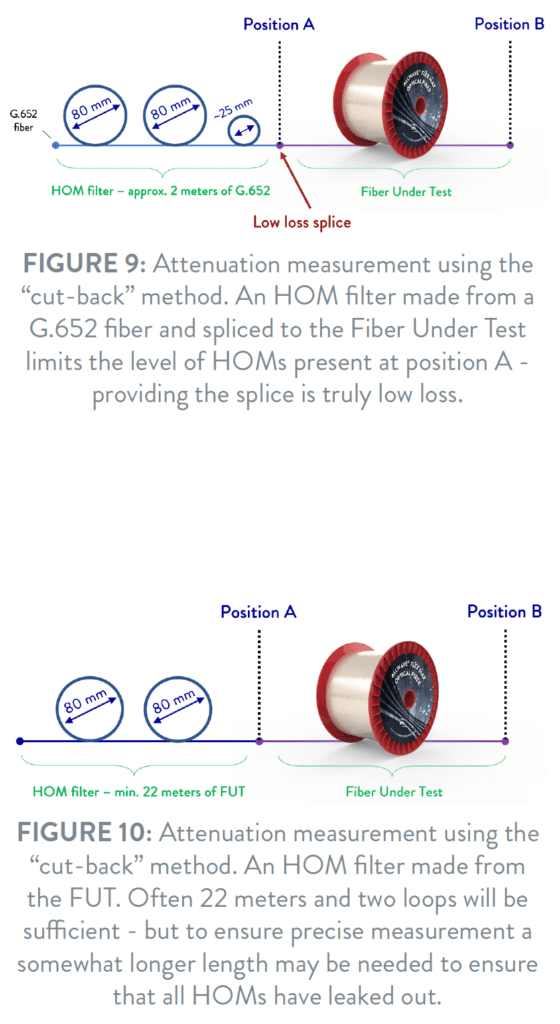
When measuring the attenuation of a Bend Insensitive fiber – including some advanced Large Area G.654 fibers – different methods may be used. The Cut Back measurement method is often considered the reference method. Light is injected into the Fiber Under Test (FUT) and the aim is to measure the power injected into the fiber (at the beginning of the fiber) and compare that to the measured power at the end of the fiber. Subtract the two and the fiber attenuation is found – divide this by the fiber length, and the attenuation in dB/km is found.
To determine the exact input power level, the fiber is often cut a short distance from the actual input end of the FUT, and the input power level is measured.
It is always important to avoid Higher Order Modes at the input of the measured fiber, since they will leak out of the FUT over a relatively short distance and be missing at the output of the FUT. HOMs are like ghosts – appearing at the input of the FUT and then disappearing along the fiber length. With these around, one would tend to measure a “too high” power level at the input of the fiber – and the resulting calculated fiber attenuation will then be too high. Such increased attenuation will tend to be more pronounced at shorter wavelengths.
Previously, such attenuation measurements were predominantly made on standard G.652 fiber and that was easy. You could grab the first 2 meters of the G.652 FUT, make the desired 2 or 3 loops directly on the fiber itself within those first 2 meters of fiber and that would give you your HOM filter and get rid of the Higher Order Modes. Your cut-back point for attenuation measurement could then be situated right after the first 2 meters of the FUT – so you would only waste 2 – 3 meters of fiber for each measurement.
But on bend insensitive fibers it is not quite as easy to get rid of the higher order modes. These fibers tend to better restrict the light from leaking out during fiber bends. Unfortunately, that is true for the higher order light modes as well – those modes which we would want to get rid of when measuring the fiber.
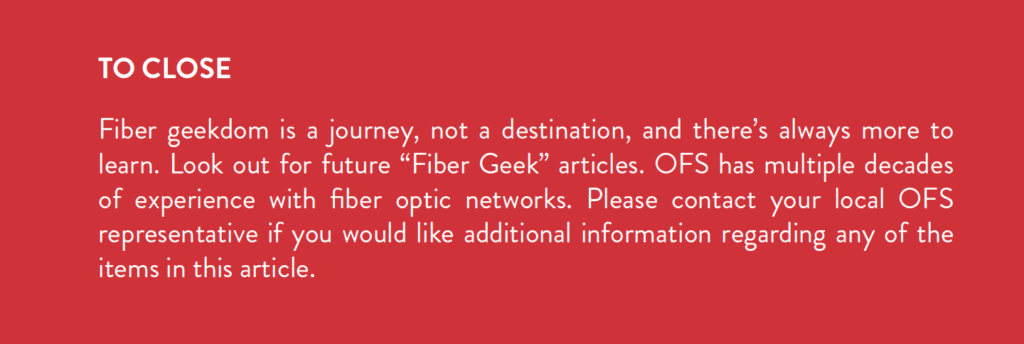
However, the 2-meter G.652 standard fiber with two 80 mm and one 25 mm loop may still be used. It may be spliced to the Fiber Under Test and if a good splice is obtained only an insignificant level of Higher Order Modes may be generated at that splice point – ensuring a good measurement if the splice point is also used as the Cut Back Point.
Another possibility is to use the first 22 meters of the FUT including the two loops of 80 mm recommended for measuring Cut-off Wavelength. Since that is the recommended test set up for COW measurement, you know that after 22 meters the HOM level is very low at the FUT’s COW or longer wavelengths. The Cut Back Point may be chosen to be just after the first 22 meters of the FUT but if very high precision measurement is required, or if FUT is relatively short, more than 22 meters may be needed.
On OTDR measurements problems caused by HOMs are often hidden. The reason for this is that an OTDR will typically have a “Dead-Zone” during which the light detector of the OTDR is recovering and as such unable to detect the incoming light signal. This may cover some 500 meters during which length the HOMs have since long leaked out of the fiber.
Tags: optical fiber